Landau Network: The Travelling Wave and Results
Podcast(Generated by NotebookLM)
My research journey began with an exploration of Partial Differential Equations (PDEs), specifically focusing on traveling wave solutions. Intrigued by the application of the Klein-Gordon equation with hyperbolic functions, I questioned the conventional use of a static beta parameter within these functions. This led me to hypothesize that a dynamically updated beta parameter, mirroring the time-dependent nature of the weight and loss function, could potentially enhance model performance.
To achieve this dynamic update, I sought a suitable function and discovered the Allen-Cahn equation through the Gemini Model. This equation, closely resembling those utilized in reaction-diffusion systems and phase-field models, offered a promising mechanism. Its ability to facilitate the propagation of “phase boundaries” through parameter space suggested potential for inducing sharp transitions within network behavior, an area requiring further investigation. Further exploration of PDE solutions for traveling waves led me to Ginzburg-Landau theory. Recognizing the potential of its free energy calculation as a component within the loss function, I pursued a simplified implementation. This resulted in a novel loss calculation framework directly inspired by a simplified Ginzburg-Landau equation.
Given the physics-based foundation of the neural network components explored thus far, I investigated the feasibility of employing a similarly grounded optimization approach. This led to the identification of Stochastic Gradient Langevin Dynamics (SGLD) as a suitable candidate. The implementation of SGLD, aided by the Claude language model, provided valuable insights into its application and divergences from traditional optimization techniques.
Preliminary results indicate comparable performance to a standard fully connected network. Although the proposed model did not consistently outperform a modified, fully connected network, this work, developed as an exploratory weekend project, provides a foundation for future research into physics-inspired neural network architectures and optimization algorithms.
Introduction: The Intersection of Physics and Machine Learning
Machine learning and physics might seem like two distinct fields, but they share a common goal: understanding and modeling complex systems. In machine learning, we build models to learn from data and make predictions. In physics, we develop theories to explain natural phenomena. By bringing these disciplines together, we can create more powerful and flexible neural networks.
The Inspiration: Ginzburg-Landau Theory
At the heart of experimental neural network lies the Ginzburg-Landau theory, a powerful framework originally developed to describe superconductivity and other phase transitions in physical systems. But what does superconductivity have to do with neural networks, you might ask?
The key insight is this: both superconducting systems and neural networks can be thought of as complex systems trying to find optimal configurations. In superconductors, it’s about finding the state of lowest energy. In neural networks, it’s about finding the configuration that best fits the data.
The Custom Loss Function: A Physics-Inspired Approach
Inspired by the Ginzburg-Landau free energy functional, we’ve designed a custom loss function for this network:
\[\mathcal{L}( \phi, \text{target} ) = \left| \text{mean} \left( \alpha (\phi_{\text{norm}} - \text{target}_{\text{norm}})^2 - \gamma (\phi_{\text{norm}} - \text{target}_{\text{norm}})^4 + 0.5 \left( \frac{\partial \phi_{\text{norm}}}{\partial x} \right)^2 \right) \right|\]Where:
- \[\phi_{\text{norm}} = \frac{\phi}{\max(|\phi|)}\]
- \[\text{target}_{\text{norm}} = \frac{\text{target\_one\_hot}}{\max(|\text{target\_one\_hot}|)}\]
- \[\frac{\partial \phi_{\text{norm}}}{\partial x} \approx \frac{\phi_{\text{norm}}(i+1) - \phi_{\text{norm}}(i-1)}{2}\]
- \(\alpha\) is the coefficient for the quadratic term that encourages the network’s output to match the target values.
- \(\gamma\) is the coefficient for the quartic term that allows for multiple stable states.
- The spatial term promotes coherence in the network’s outputs across spatial dimensions.
Breakdown of the Loss Function
- Quadratic Term: Encourages the network’s output to match the target values. This is similar to the traditional mean squared error used in many neural networks.
- Quartic Term: Allows for multiple stable states, potentially enabling the network to capture more complex patterns. This term, with a negative sign, adds richness to the energy landscape, facilitating better exploration during training.
- Spatial Term: Promotes coherence in the network’s outputs across spatial dimensions. This is particularly useful for tasks involving spatial data, such as image processing.
Dynamic Weight Modification: Adapting to Input
Another unique feature of this network is its dynamic weight modification scheme:
\[\mathbf{W} = \mathbf{W}_0 \cdot \left( \cosh(5\beta) \cdot \mathbf{a} + t_{\text{dynamic}} \cdot \sinh(5\beta) \right)\]where:
- \(\mathbf{W}_0\) is the initial weight matrix.
- \(\beta\) is a learned parameter.
- \(t_{\text{dynamic}}\) is a dynamic term that adapts based on the input.
Explanation
This might look complex, but the idea is simple yet powerful: the network adapts its weights based on the input it receives. The use of hyperbolic functions (cosh and sinh) introduces a form of non-Euclidean geometry, potentially allowing the network to better capture hierarchical structures in the data.
Physics-Inspired Optimization: Langevin Dynamics
To train this network, I’ve developed a custom optimizer inspired by Langevin dynamics, a concept from statistical physics used to describe the motion of particles in a fluid:
Step Method Equation
For each parameter \(\theta_i\):
-
Compute the loss gradient with respect to each parameter: \(F_i = -\frac{\partial \mathcal{L}}{\partial \theta_i}\) where \(\mathcal{L}\) is the loss function, and \(F_i\) is the force (negative gradient) applied to \(\theta_i\).
-
Update the velocity: \(v_i \leftarrow (1 - \gamma) v_i + \alpha F_i + \sqrt{2 \gamma \alpha T} \cdot \eta_i\) where \(\eta_i\) is a noise term sampled from a standard normal distribution \(\mathcal{N}(0, 1)\).
-
Update the parameter: \(\theta_i \leftarrow \theta_i + v_i\)
Full Update Equation
For each parameter \(\theta_i\) :
\[v_i \leftarrow (1 - \gamma) v_i - \alpha \frac{\partial \mathcal{L}}{\partial \theta_i} + \sqrt{2 \gamma \alpha T} \cdot \eta_i\] \[\theta_i \leftarrow \theta_i + v_i\]Where:
- \(\alpha\) is the learning rate.
- \(\gamma\) is the damping coefficient.
- \(T\) is the temperature.
- \(\eta_i \sim \mathcal{N}(0, 1)\) is the noise term.
Combined in a Single Expression
Combining both steps, we get the following update rules for each parameter \(\theta_i\):
\[v_i \leftarrow (1 - \gamma) v_i - \alpha \frac{\partial \mathcal{L}}{\partial \theta_i} + \sqrt{2 \gamma \alpha T} \cdot \eta_i\] \[\theta_i \leftarrow \theta_i + v_i\]This optimizer introduces concepts of velocity, damping, and temperature into the learning process. The idea is to allow the network to explore the loss landscape more thoroughly, potentially escaping local minima and finding better global solutions.
Beta Update Equations
Given:
- \(\beta\) is the learnable parameter.
- \(\phi\) is the model output.
- \(\text{target}\) is the ground truth.
- \(dt\) is the time step.
- \(\kappa\) is a constant.
The steps involved in updating \(\beta\) are as follows:
-
Compute the loss derivative with respect to the input: \(\text{d\_loss} = \mathcal{L}(\phi, \text{target})\) where \(\mathcal{L}\) is the loss function.
-
Compute the spatial derivative of the loss: \(\text{d\_loss}_x = \frac{\text{d\_loss}_{i+1} - \text{d\_loss}_{i-1}}{2}\)
-
Compute the force term: \(\text{force} = -\kappa \cdot \text{d\_loss}_x\)
-
Compute the second spatial derivative of \(\beta\): \(\beta_{xx} = \beta_{i+1} - 2\beta_i + \beta_{i-1}\)
-
Compute the time derivative of \(\beta\): \(\beta_t = \frac{\beta - \beta_{\text{previous}}}{dt}\)
-
Update \(\beta\) using the combined terms: \(\beta \leftarrow \beta + dt \left( \beta_t - \beta_{xx} + \beta - \beta^3 + \text{force} \right)\)
Putting these steps together, the beta update rule can be written as:
\[\beta_{t+1} \leftarrow \beta_t + dt \left( \frac{\beta_t - \beta_{t-1}}{dt} - (\beta_{i+1} - 2\beta_i + \beta_{i-1}) + \beta - \beta^3 - \kappa \cdot \frac{\text{d\_loss}_{i+1} - \text{d\_loss}_{i-1}}{2} \right)\]Putting It All Together: A New Paradigm for Neural Networks
By combining these physics-inspired components - the Ginzburg-Landau-based loss function, dynamic weight modification, and Langevin dynamics-inspired optimization - i’ve created a neural network that operates on principles quite different from traditional architectures.
Potential Benefits
- Better Handling of Complex, Hierarchical Data Structures: The dynamic weight modification and rich energy landscape help capture intricate patterns in the data.
- Improved Exploration of the Solution Space: The Langevin dynamics-inspired optimizer enhances the network’s ability to find global optima.
- Multiple Stable States: The quartic term allows for capturing diverse data patterns.
- Enhanced Spatial Coherence: Useful for tasks involving spatial data, ensuring smooth transitions in the output.
Challenges
- Increased Complexity in Training: More parameters and terms to tune can complicate the training process.
- Need for Careful Interpretation: Understanding the network’s behavior requires a deeper theoretical insight.
- Potential Instabilities: Non-standard loss functions and optimization processes might introduce new challenges.
Experimental Results
Example Outputs from 1 Layer Experimental NN
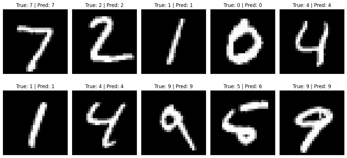
1 Layer Experimental Net Example Test Set Output
To provide a clear comparison, here’s how this experimental neural network performs on MNIST dataset across various metrics:

1 Layer Experimental NN with Mish activation and batch norm

2 Layer Experimental NN with Mish activation and batch norm
| Metric | 1 Layer | 2 Layer |
|---|---|---|
| Accuracy on MNIST | 92% | 96% |
| Epoch | 100 epochs | 100 epochs |
| alpha | 0.0095 | 0.0095 |
| gamma | 6.5 | 6.5 |
| beta init | 1e-3 | 1e-3 |
| learning rate | 1e-2 | 1e-2 |
| kappa | 1e-2 | 1e-2 |
| hidden layer | - | 156 |
| damping | 0.001 | 0.001 |
| temperature | 0.008 | 0.008 |
| dt | 0.001 | 0.001 |
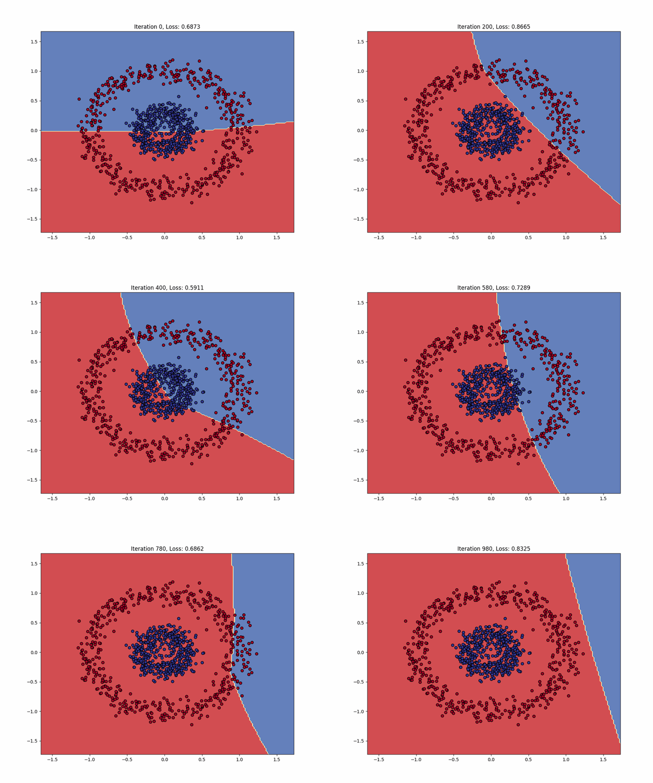
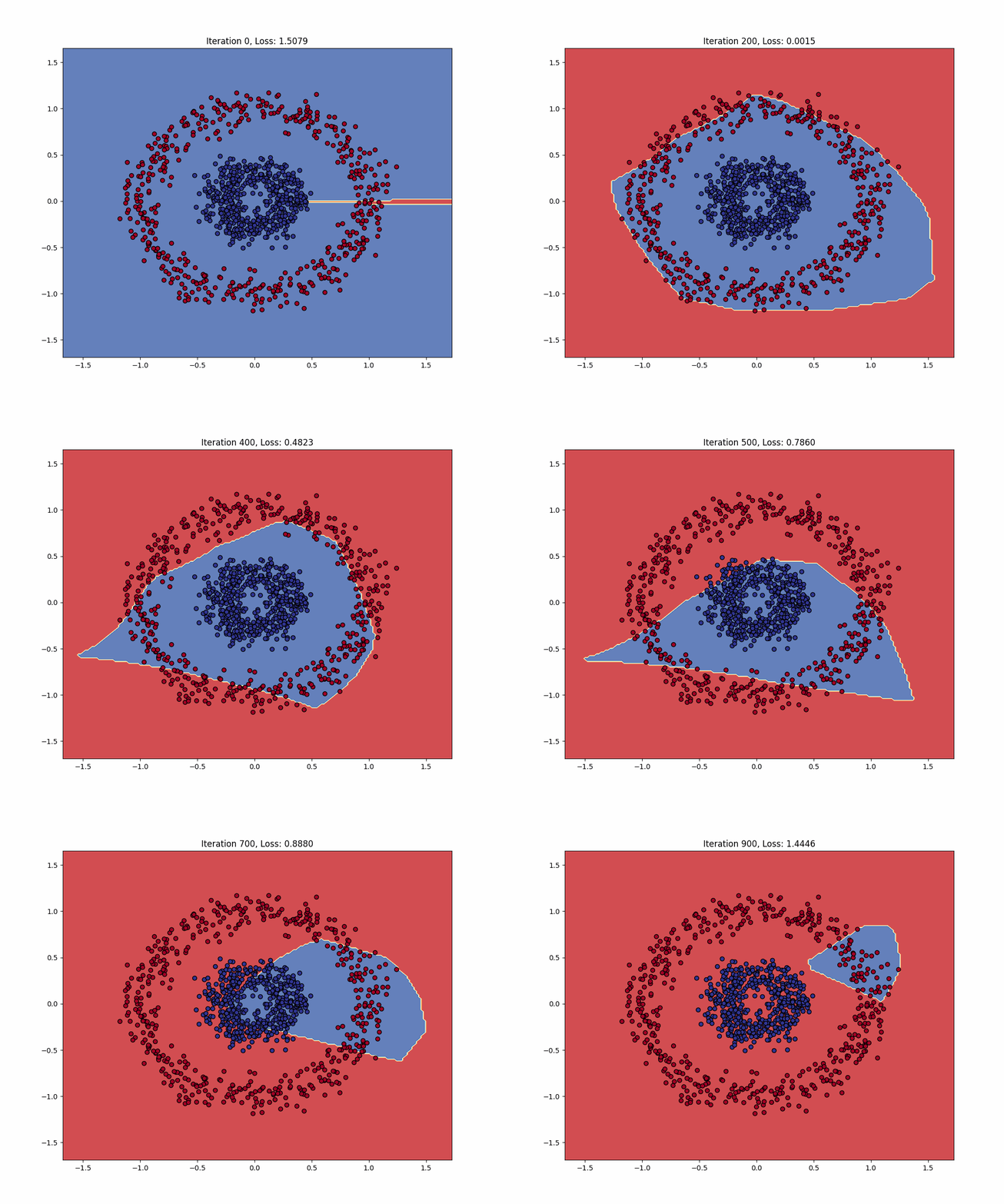
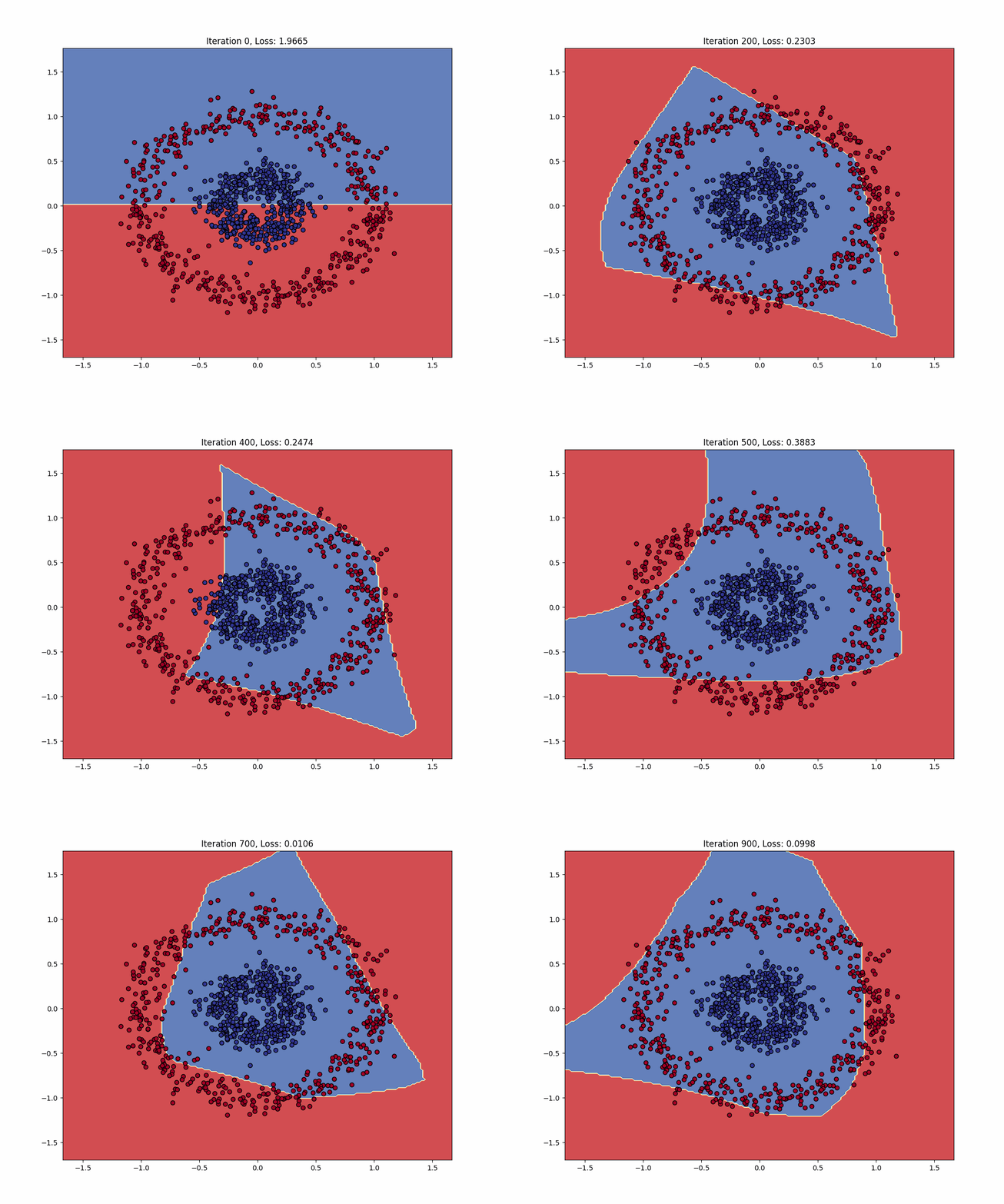
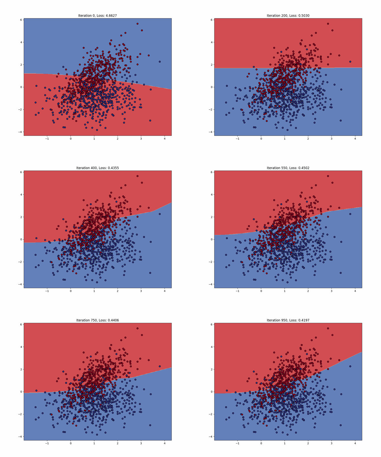
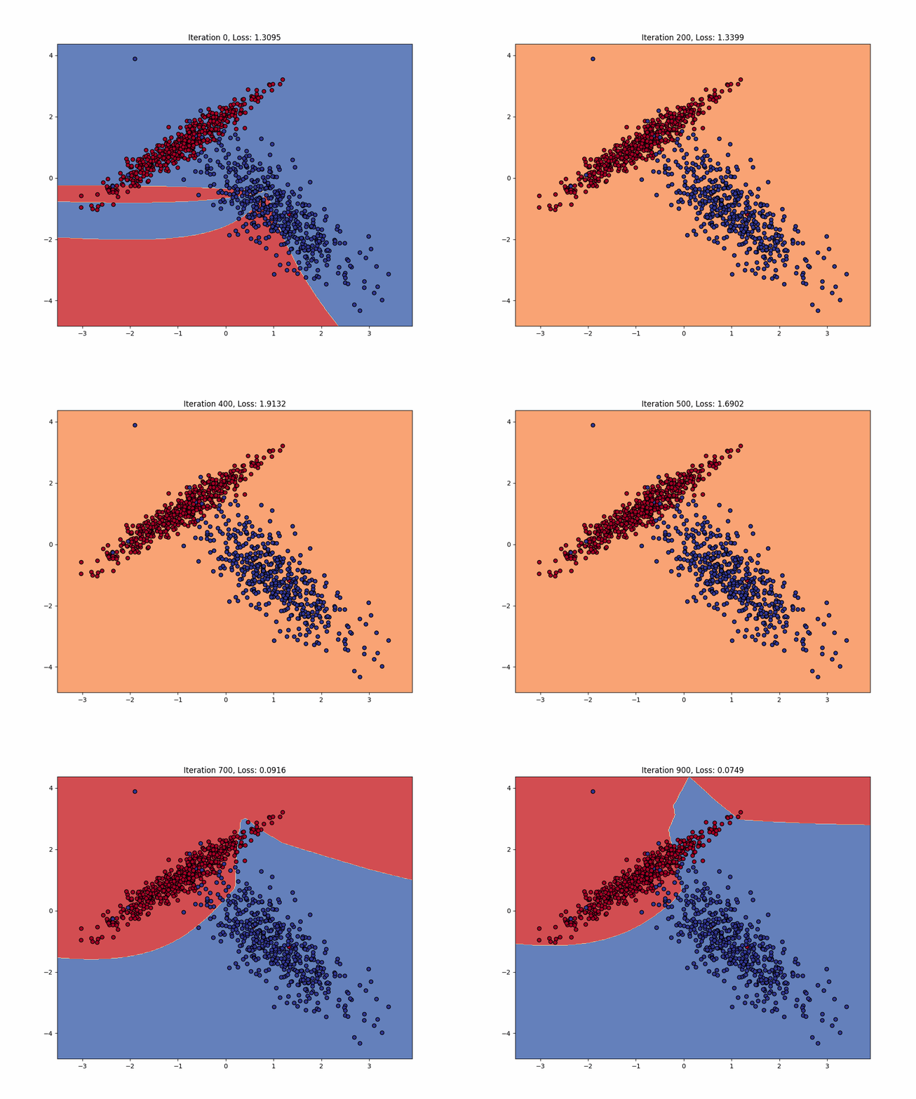
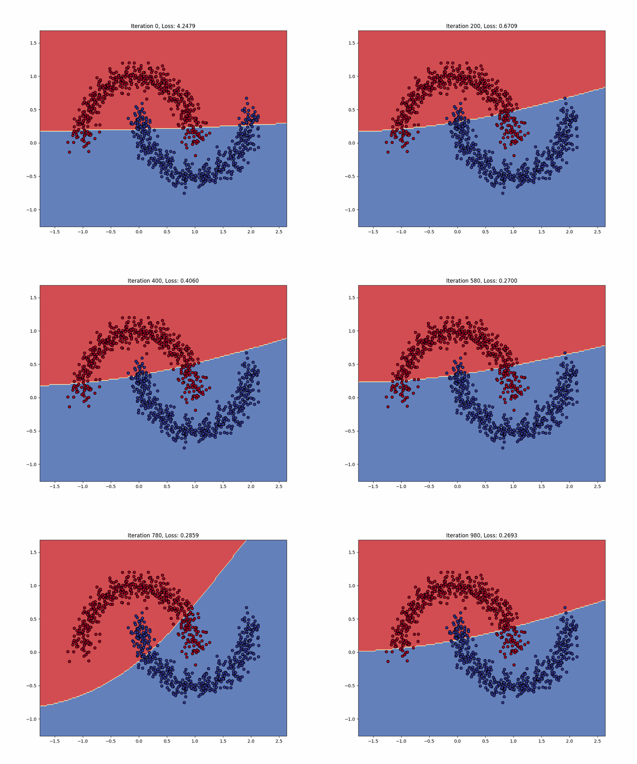
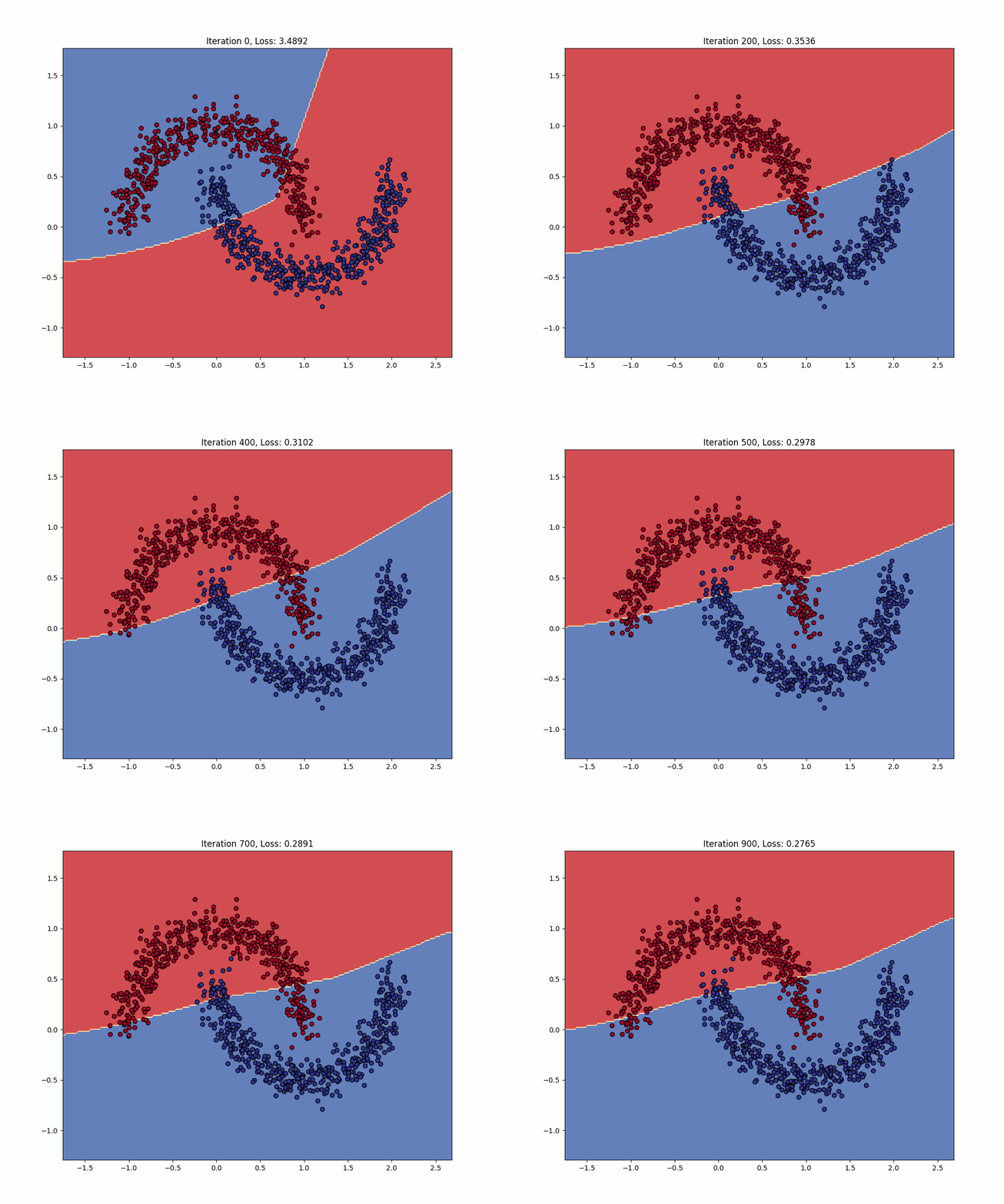
Visualization with Some Datasets
1 Layer Example on Circle dataset
2 Layer Example on Circle dataset
2 Layer Example on Circle dataset
1 Layer Example on Classification dataset
1 Layer Example on Classification dataset
1 Layer Example on Moons dataset
2 Layer Example on Moons dataset
Code Snippet for the ExperimentalLayer
Here’s a more detailed code snippet of the ExperimentalLayer to give readers a clearer picture of its implementation:
Landau Layer with Traveling Wave Approach
class LandauLayer(nn.Module):
    def __init__(self, input_size, output_size, beta_init, alpha=0.0035, gamma=5.0):
        super(LandauLayer, self).__init__()
        self.w = nn.Parameter(torch.randn(output_size, input_size))
        nn.init.xavier_normal_(self.w)
        self.beta = nn.Parameter(torch.tensor(beta_init).float())
        self.alpha = alpha
        self.gamma = gamma
        self.t = nn.Parameter(torch.tensor([1.0]))

    def forward(self, x):
        t_dynamic = self.t * torch.sigmoid(torch.mean(x, dim=-1)).unsqueeze(-1)
        w2 = self.w * (torch.arange(x.size(-1), dtype=torch.float, device=x.device) * torch.cosh(5 * self.beta) + t_dynamic * torch.sinh(5 * self.beta)).unsqueeze(1)
        phi = torch.matmul(w2, x.unsqueeze(-1)).squeeze(-1)
        return phi

    def update_beta(self, phi, target, dt, kappa=0.01):
        d_loss = self.d_loss(phi, target).detach()
        d_loss_x = (torch.roll(d_loss, -1) - torch.roll(d_loss, 1)) / 2.0
        force = -kappa * d_loss_x

        with torch.no_grad():
            beta_xx = (torch.roll(self.beta, -1) - 2 * self.beta + torch.roll(self.beta, 1))
            beta_t = (self.beta - self.beta.clone().detach()) / dt
            self.beta.data += dt * (beta_t - beta_xx + self.beta - self.beta**3 + force)

    def d_loss(self, phi, target):
        max_abs_phi = torch.max(torch.abs(phi), dim=1, keepdim=True)[0]
        phi_norm = phi / (max_abs_phi)

        phi_x = (torch.roll(phi_norm, -1, dims=0) - torch.roll(phi_norm, 1, dims=0)) / 2.0
        target_one_hot = F.one_hot(target, num_classes=phi.size(1)).float()

        max_abs_target = torch.max(torch.abs(target_one_hot), dim=1, keepdim=True)[0]
        target_norm = target_one_hot / (max_abs_target )

        diff = phi_norm - target_norm

        quadratic_term = self.alpha * (diff)**2
        quartic_term = self.gamma * (diff)**4
        spatial_term = 0.5 * phi_x**2

        d_loss = quadratic_term - quartic_term + spatial_term

        mean_d_loss = d_loss.mean()
        return torch.abs(mean_d_loss)
Modified Langevin Optimizer
class LangevinLandauOptimizer:
    def __init__(self, model, learning_rate=0.001, damping=0.1, temperature=0.8):
        self.model = model
        self.lr = learning_rate
        self.damping = damping
        self.temperature = temperature
        self.velocities = [torch.zeros_like(p.data) for p in model.parameters()]

    def step(self, phi, target):
        d_loss = self.model.llayer2.d_loss(phi, target)

        for i, (param, velocity) in enumerate(zip(self.model.parameters(), self.velocities)):
            force = -torch.autograd.grad(d_loss, param, create_graph=True)[0]

            # Langevin dynamics directly application without modify
            velocity.mul_(1 - self.damping).add_(force * self.lr)
            noise_scale = torch.sqrt(torch.tensor(2 * self.damping * self.temperature * self.lr))
            velocity.add_(torch.randn_like(velocity) * noise_scale)

            param.data.add_(velocity)

        return d_loss.item()
Simple Network
class ExperimentalNet(nn.Module):
    def __init__(self, input_size, hidden_size, output_size, beta_init):
        super(ExperimentalNet, self).__init__()
        self.llayer1 = LandauLayer(input_size, hidden_size, beta_init)
        self.llayer2 = LandauLayer(hidden_size, output_size, beta_init)
        self.bn1 = nn.BatchNorm1d(hidden_size)

    def forward(self, x):
        # x = F.rrelu(self.bn1(self.layer1(x)))
        x = F.rrelu(self.bn1 (self.llayer1(x)))
        x = F.rrelu(self.llayer2(x))
        return x